Tutorial
The example in this tutorial is a good approximation to a real physical situation, namely a Cesium-133 atom in an addressable optical lattice. Alkali atoms in optical lattices are one of the proposed methods of realizing a quantum computer. This particular example is a simulation of a one-qubit gate--a "flip" or NOT gate (equivalently, a rotation by pi about the X axis, in the Bloch sphere picture).
This tutorial covers the following topics:
[Simulation Details] [Basic Parameters] [Initial State] [Potentials] [Energy and Time Parameters] [Output Options] [Graphing and Visualization]
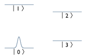 In the simulation example, the atom has one degree of motional freedom, and four possible internal states ("levels"). The levels are a subset of the hyperfine sublevels of the 6 2S1/2 state. Specifically, the levels are mF=0 F=3 and F=4 (labeled |0> and |1>), and mF=1 F=4 and F=3 (labeled |3> and |4>), as shown in the figure on the right. The atom experiences a state-dependent potential, with all states experiencing a harmonic trapping potential. |3> also is subject to a small Gaussian-shaped trapping potential, while |4> experiences a Gaussian anti-trapping potential (e.g. same in magnitude but opposite in sign to that experienced by |3>. Physically, these Gaussian terms would be the result of an AC Stark Shift (or "light shift") due to an "addressing" laser focused on this particular atom. There are also time-dependent couplings between the levels, which would be generated by appropriate microwave pulses in an actual experiment.
The units used in this tutorial are "atomic units", e.g. energy is given in Hartrees, lengths are specified in multiples of the Bohr Radius, time is in units of hbar / Hartree, and mass is multiples of the electron mass. qsims is unit-agnostic--you are free to use whatever units you want with qsims. Just specify the appropriate values for hbar and other constants when asked.
Starting qsims
Now, to begin the tutorial. Launch qsims from the command line with the "-i" option to enter interactive mode. You can also use "-f filename" to read input from a file, "-p parameters" to use the parameters given on the command line, or "-h" for help. Upon launch, qsims displays a short blurb about the GNU General Public License, which is the license under which qsims is distributed.
% qsims -i
qsims v0.4 Copyright (c) 2004 Travis Beals, Built Mar 2 2005
qsims comes with ABSOLUTELY NO WARRANTY. qsims is free software,
and you are welcome to redistribute it under certain conditions.
See the GNU General Public License 2 (or any later version) for details.
Next, enter the value of hbar (which is 1 in atomic units), and the mass of the atom. The mass is used when calculating the kinetic term in the Hamiltonian, and also in harmonic potentials.
* Physical parameters
- Enter hbar:
1
- Enter mass:
242272
Now we have to enter some simulation parameters. First is the number of levels (i.e. internal states of the atom). Then, enter the number of motional degrees of freedom (e.g. dimensions). Next, enter the number of grid points used in the discretization of the spatial wavefunction, for each dimension (hint: powers of two are good, as are products of powers of small prime numbers). Finally, enter the length interval dx, or alternatively, if your potential is going to be roughly harmonic, enter -omega (where omega is the angular frequency of the harmonic potential) to have an optimal value for dx automatically calculated.
* Grid parameters
- Enter number of levels:
4
- Enter number of dimensions:
1
+ Enter length of dimension 0:
256
- Enter dx, or -omega to have dx calculated automatically:
-2.4042e-12
Here we specify the initial state. We do this by specifying a state for each level, giving the states in terms of harmonic oscillator eigenstates (this means we have to tell qsims what omega to use when generating the harmonic oscillator eigenstates--yes, you have to enter omega again, since you could conceivably want a different omega). After we enter the omega, we're asked to enter the number of superimposed states, which is just the number of harmonic oscillator eigenstates we sum over to get the initial state for this particular level. Next, specify the complex coefficient for each eigenstate, as well as the corresponding eigenvalue for each axis (i.e. if we were working in three dimensions, you need to give three numbers to describe a particular harmonic oscillator eigenstate). In the example, we just have the ground state, so the coefficient is 1.0 + 0.0 i (which we enter as 1 0), and the eigenvalue is of course 0. Finally, specify the displacement of the eigenstate from the origin along each axis (probably you're just going to want to enter 0).
* Initial States
- Initial state for level 0
+ Enter omega:
2.4042e-12
+ Enter the number of superimposed states:
1
- Enter the complex normalization "re im" for state 0:
1 0
- Enter harmonic oscillator eigenstate for axis 0:
0
- Enter displacement of harmonic oscillator along axis 0:
0
Now that we've specified the state for the level |0> as the harmonic oscillator ground state, we set the initial state for the remaining levels to 0.
- Initial state for level 1
+ Enter omega:
2.4042e-12
+ Enter the number of superimposed states:
0
- Initial state for level 2
+ Enter omega:
2.4042e-12
+ Enter the number of superimposed states:
0
- Initial state for level 3
+ Enter omega:
2.4042e-12
+ Enter the number of superimposed states:
0
Next come the potentials and couplings. Couplings are treated equivalently to potentials--the only difference is that "potentials" are diagonal terms in the Hamiltonian (in the "level" representation), whereas "couplings" are off-diagonal terms. We choose a type of potential--in this case, harmonic. Next, we specify omega, then enter 0 to indicate that this particular potential is not time-dependent. Finally, we specify the target levels for this potential. In this case, we want the levels |0> and |1> to experience this potential, so we enter 0 0, then 1 1, then -1 to indicate that we're done.
* Potentials
- Select a type of potential:
0) Composite
1) Flat
2) Harmonic
3) Gaussian
-1) Done
2
+ Enter omega:
2.4042e-12
+ Time dependent scaling? 0) No 1) Yes (start with scaling=0) 2) Yes (start with scaling=1):
0
+ Enter target levels in form "a b", or -1 to finish:
0 0
+ Enter target levels in form "a b", or -1 to finish:
1 1
+ Enter target levels in form "a b", or -1 to finish:
-1
Now things get trickier--we're going to specify a composite potential, which is a sum of other potential types. Composite potentials can even contain other composite potentials, although the circumstances under which this is useful are uncommon. Once you select the "Composite" type, you then specify each of the component potentials in the same manner as before.
- Select a type of potential:
0) Composite
1) Flat
2) Harmonic
3) Gaussian
-1) Done
0
Here comes the first component of the composite potential--we're going to specify a Gaussian potential. Gaussian potentials have a mean (which is technically a vector, so you must enter the component of the vector for each dimension), a standard deviation, and an amplitude. This Gaussian won't be time-dependent.
+ Enter a component of the composite function
- Select a type of potential:
0) Composite
1) Flat
2) Harmonic
3) Gaussian
-1) Done
3
+ Enter the mean (mu) for dimension 0:
0
+ Enter the standard deviation (sigma):
11338.4
+ Enter the amplitude (value at x = mu):
1.92076e-11
+ Time dependent scaling? 0) No 1) Yes (start with scaling=0) 2) Yes (start with scaling=1):
0
Now for the next component of the composite potential--a constant (flat) function. This one's pretty straightforward.
+ Enter a component of the composite function
- Select a type of potential:
0) Composite
1) Flat
2) Harmonic
3) Gaussian
-1) Done
1
+ Enter the constant in form "re im":
6.25018e-14 0
+ Time dependent scaling? 0) No 1) Yes (start with scaling=0) 2) Yes (start with scaling=1):
0
Here's another constant function. Yes, this could have simply been added to the previous constant, but it was kept separate for conceptual clarity (notice that this function exactly offsets the value of the Gaussian function at the origin).
+ Enter a component of the composite function
- Select a type of potential:
0) Composite
1) Flat
2) Harmonic
3) Gaussian
-1) Done
1
+ Enter the constant in form "re im":
-1.92076e-11 0
+ Time dependent scaling? 0) No 1) Yes (start with scaling=0) 2) Yes (start with scaling=1):
0
Now we add a harmonic term, with the same omega as the harmonic potential we used for |0> and |1>. After that, we're finished entering components for the composite potential, so we enter "-1" for "done".
+ Enter a component of the composite function
- Select a type of potential:
0) Composite
1) Flat
2) Harmonic
3) Gaussian
-1) Done
2
+ Enter omega:
2.4042e-12
+ Time dependent scaling? 0) No 1) Yes (start with scaling=0) 2) Yes (start with scaling=1):
0
+ Enter a component of the composite function
- Select a type of potential:
0) Composite
1) Flat
2) Harmonic
3) Gaussian
-1) Done
-1
We now tell qsims that the composite function should not have any overall time dependence (note that individual components could still be time dependent), and set |3> as the target level.
+ Time dependent scaling? 0) No 1) Yes (start with scaling=0) 2) Yes (start with scaling=1):
0
+ Enter target levels in form "a b", or -1 to finish:
3 3
+ Enter target levels in form "a b", or -1 to finish:
-1
We go through the same composite function exercise for |2>. The only difference is that the amplitude of the Gaussian now has the opposite sign.
- Select a type of potential:
0) Composite
1) Flat
2) Harmonic
3) Gaussian
-1) Done
0
+ Enter a component of the composite function
- Select a type of potential:
0) Composite
1) Flat
2) Harmonic
3) Gaussian
-1) Done
3
+ Enter the mean (mu) for dimension 0:
0
+ Enter the standard deviation (sigma):
11338.4
+ Enter the amplitude (value at x = mu):
-1.92076e-11
+ Time dependent scaling? 0) No 1) Yes (start with scaling=0) 2) Yes (start with scaling=1):
0
+ Enter a component of the composite function
- Select a type of potential:
0) Composite
1) Flat
2) Harmonic
3) Gaussian
-1) Done
1
+ Enter the constant in form "re im":
-6.5935e-14 0
+ Time dependent scaling? 0) No 1) Yes (start with scaling=0) 2) Yes (start with scaling=1):
0
+ Enter a component of the composite function
- Select a type of potential:
0) Composite
1) Flat
2) Harmonic
3) Gaussian
-1) Done
1
+ Enter the constant in form "re im":
1.92076e-11 0
+ Time dependent scaling? 0) No 1) Yes (start with scaling=0) 2) Yes (start with scaling=1):
0
+ Enter a component of the composite function
- Select a type of potential:
0) Composite
1) Flat
2) Harmonic
3) Gaussian
-1) Done
2
+ Enter omega:
2.4042e-12
+ Time dependent scaling? 0) No 1) Yes (start with scaling=0) 2) Yes (start with scaling=1):
0
+ Enter a component of the composite function
- Select a type of potential:
0) Composite
1) Flat
2) Harmonic
3) Gaussian
-1) Done
-1
+ Time dependent scaling? 0) No 1) Yes (start with scaling=0) 2) Yes (start with scaling=1):
0
+ Enter target levels in form "a b", or -1 to finish:
2 2
+ Enter target levels in form "a b", or -1 to finish:
-1
Now we're going to specify some time-dependent couplings. This first one will couple |0> to |2>, and also |1> to |3>. The coupling does not depend on the spatial position of the atom, so we choose a flat potential, and set an appropriate constant.
- Select a type of potential:
0) Composite
1) Flat
2) Harmonic
3) Gaussian
-1) Done
1
+ Enter the constant in form "re im":
0.866025e-12 0
We tell qsims to make the coupling time-dependent, and start with 0 coupling. Then we specify the first time step. To do this, we enter the start time for the time step, the ramping-up time (the time over which the potential will linearly change from its previous value to the new value), and the scaling factor (the multiple of the default value to which the function gets scaled).
+ Time dependent scaling? 0) No 1) Yes (start with scaling=0) 2) Yes (start with scaling=1):
1
* Scaling time step start time?
1.30671e+12
* Scaling ramping-up time?
0
* Scaling factor?
1
We still need to add more time steps, so we repeat the process.
* Add another time step? 0) No 1) Yes
1
* Scaling time step start time?
4.4483e+12
* Scaling ramping-up time?
0
* Scaling factor?
0
* Add another time step? 0) No 1) Yes
0
Now we set the target levels. Since we want to couple |0> to |2>, we enter 0 2, then 2 0. We do similarly for |1> and |3>.
+ Enter target levels in form "a b", or -1 to finish:
0 2
+ Enter target levels in form "a b", or -1 to finish:
2 0
+ Enter target levels in form "a b", or -1 to finish:
1 3
+ Enter target levels in form "a b", or -1 to finish:
3 1
+ Enter target levels in form "a b", or -1 to finish:
-1
We now create another time-dependent coupling, this one between |2> and |3>. Finally, we enter "-1" to indicate that we're finished specifying potentials and couplings.
- Select a type of potential:
0) Composite
1) Flat
2) Harmonic
3) Gaussian
-1) Done
1
+ Enter the constant in form "re im":
1e-12 0
+ Time dependent scaling? 0) No 1) Yes (start with scaling=0) 2) Yes (start with scaling=1):
1
* Scaling time step start time?
1.30671e+12
* Scaling ramping-up time?
0
* Scaling factor?
1
* Add another time step? 0) No 1) Yes
1
* Scaling time step start time?
4.4483e+12
* Scaling ramping-up time?
0
* Scaling factor?
0
* Add another time step? 0) No 1) Yes
0
+ Enter target levels in form "a b", or -1 to finish:
2 3
+ Enter target levels in form "a b", or -1 to finish:
3 2
+ Enter target levels in form "a b", or -1 to finish:
-1
- Select a type of potential:
0) Composite
1) Flat
2) Harmonic
3) Gaussian
-1) Done
-1
We now specify the minimum energy (Emin), the energy range (dE = Emax - Emin), and the time step (dt). Generally, for stability, the range should be set to much larger than the true energy range, as any state with an energy outside the specified energy may cause the simulation to diverge. There is a tradeoff between dE and the computational cost of calculating a time step, so experiment to find a good value.
* Simulation Parameters
- Enter dE (Emax - Emin):
1.5e-8
- Enter Emin:
-5e-9
- Enter dt:
2.55217e+9
We then pick the number of time steps, thus determining the length of time simulated. Also, the number of recursion steps in the Chebychev expansion can be manually set, or "-1" can be entered to allow qsims to automatically choose the number of recursion steps.
- Enter number of timesteps:
1800
- Enter number of recursion steps (-1 for automatic):
-1
All that remains is to set output options for the simulation. A simple text-based progress display can be enabled if desired, although this does slightly slow down the simulation. A variety of output-to-file options are available, including outputting the "grid" (the discretized wavefunction) at fixed intervals, and / or performing a decomposition of the final state into harmonic oscillator eigenstates. If either file output option is chosen, a path must be specified to a directory into which the files should be placed, and a base name must be given for the files. For example, if the base name is "test", then files "test.0.0.txt", "test.1.0.txt", ... , "test.3.0.txt", "test.0.1.txt", ..., "test.3.1.txt", "test.0.2.txt", etc. will be created. The first number after "test" is the level, while the second is the time step--one file is created per level per time step.
* Output Options
- Would you like a progress display?
0) No
1) Yes
0
- What file output would you like?
0) No output
1) Grid output
2) Harmonic Oscillator Eigenstate Decomposition
3) Both
3
0)+ Enter the period of grid output to file (once every x time steps):
4
0)+ Enter the omega to use for H.O. eigenstate decomposition:
2.4042e-12
0)+ Enter base pathname (full path, using "/" as the directory separator, no spaces):
/full/path/to/target/directory/
0)+ Enter base filename (no spaces):
myBaseName
qsims then outputs a string of all the parameters you chose. This string can be used as input (either in a file or via the "-p" option) for future runs of qsims.
Simulation parameters:
1 242272 4 1 256 -2.4042e-12 2.4042e-12 1 1 0 0 0 2.4042e-12 0 2.4042e-12 0 2.4042e-12 0 2 2.4042e-12 0 0 0 1 1 -1 0 3 0 11338.4 1.92076e-11 0 1 6.25018e-14 0 0 1 -1.92076e-11 0 0 2 2.4042e-12 0 -1 0 3 3 -1 0 3 0 11338.4 -1.92076e-11 0 1 -6.5935e-14 0 0 1 1.92076e-11 0 0 2 2.4042e-12 0 -1 0 2 2 -1 1 8.66025e-13 0 1 1.30671e+12 0 1 1 4.4483e+12 0 0 0 0 2 2 0 1 3 3 1 -1 1 1e-12 0 1 1.30671e+12 0 1 1 4.4483e+12 0 0 0 2 3 3 2 -1 -1 1.5e-08 -5e-09 2.55217e+09 1800 -1 0 3 4 2.4042e-12 /full/path/to/target/directory/ someBaseName
Now you just wait while qsims performs the simulation.
Once the simulation is done, you may want to generate a movie from the output files (assuming you chose "Grid output"). Graphs of each grid file can be produced with GNUPLOT, and combined into a movie with a program like ffmpeg. qsims automatically generates a file "myBaseName.script" which contains GNUPLOT commands for plotting each output file:
call 'plotit.script' 0 "myBaseName.0.png" "myBaseName.0.0.txt" "myBaseName.0.1.txt" "myBaseName.0.2.txt" "myBaseName.0.3.txt"
call 'plotit.script' 1 "myBaseName.1.png" "myBaseName.1.0.txt" "myBaseName.1.1.txt" "myBaseName.1.2.txt" "myBaseName.1.3.txt"
The script can be run by typing gnuplot myBaseName.script on the command line while in the directory containing the output files, or by typing load 'myBaseName.script' from within GNUPLOT (which must have been launched from within the output file directory). The script expects to find another script in the same directory, with the name "plotit.script". This script must take the correct number of arguments (two plus the number of levels, so five in this case), where the first is the time step number, the second the name of the image file to output, and the remainder are names of "grid" files from qsims. An example of a possible plotting script is given below:
set terminal push

set terminal png notransparent medium size 1024,768

set output "$1"


set key off

unset border

unset xtics

unset ytics

set yrange [0:0.04]

set style line 1 lt 20 lw 4 pt -1


set rmargin 0.0

set lmargin 0.0

set tmargin 0.0

set bmargin 0.0


set multiplot

set size ratio 0.75 0.4,0.3

set origin 0.1,0.1

plot [64:192] '$2' using 1 ls 1 smooth csplines


set origin 0.6,0.2

plot [64:192] '$5' using 1 ls 1 smooth csplines


set origin 0.6,0.6

plot [64:192] '$4' using 1 ls 1 smooth csplines


set origin 0.1,0.7

plot [64:192] '$3' using 1 ls 1 smooth csplines

set size noratio 1,1

unset multiplot


set terminal pop

unset output
The resulting image files could then be converted into an mpeg movie with ffmpeg via the following command (typed as a single line):
ffmpeg -i myBaseName.%d.png -title "One qubit gate" -author "Me" -s 640x426 -croptop 54 -b 1000 -vcodec mpeg4 myBaseName.mov
qsims is hosted by
 |
Last updated 6 April 2005
by Travis Beals. |